


Posted in January 2015
A project is complete when it starts working for you
“A project is complete when it starts working for you, rather than you working for it.”
-Scott Allen
January has been a month with extensive activities outside the lecture halls. I had couple of lectures in the first week of January after the Christmas break. After that I wrapped up the course projects for Q2 before heading into the exams.
For the handwritten Digit Classification project for Pattern recognition, we had to edit the report as we had completed the implementation in December. On the other hand, we began the assignment for Filtering and System Identification course in the second week of January and had to do a quick work as we did not have much time. We analysed the given data input and outputs, pre-processed it and eliminated datasets that we thought were not appropriately recorded (in terms of the duration of recording, sampling frequency and the amount of noise). We then used Past Output Multivariable Output Error State Space algorithm (PO-MOESP) to find the system matrices as well as validated our choice through Variance Accounted For (VAF).
The project that took up maximum time was the Image Segmentation project. It has certainly widened my knowledge in the field and it was an enriching experience. The project was an implementation of http://www.cs.berkeley.edu/~malik/papers/arbelaezMFM-pami2010.pdf. We performed contour detection using Local Cues such as brightness, colour and texture by splitting the image into four channels. We made use of Oriented Gradients in each of the channels in eight orientations [0,pi) before choosing the maximum value over the orientations for all channels for each pixel. In the texture channel, k-means clustering was used in order to obtain the textons. In order to include global information, we performed Spectral Clustering. As we did not have closed contours at all times, we performed Hierarchical Segmentation, wherein Watershed Segmentation was extended to Oriented Watershed Transform. Finally we used Ultrametric Contour Mapping. The images from different steps can be seen below.
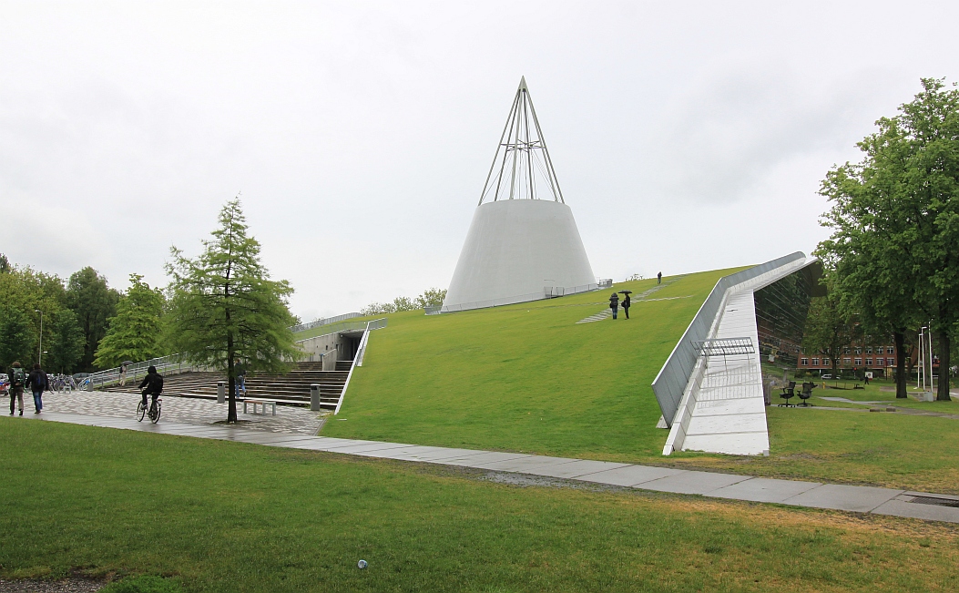
Original Image
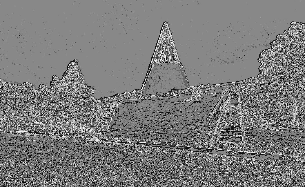
Texture image
Multiscale Oriented Gradients (using the max value over the orientations)
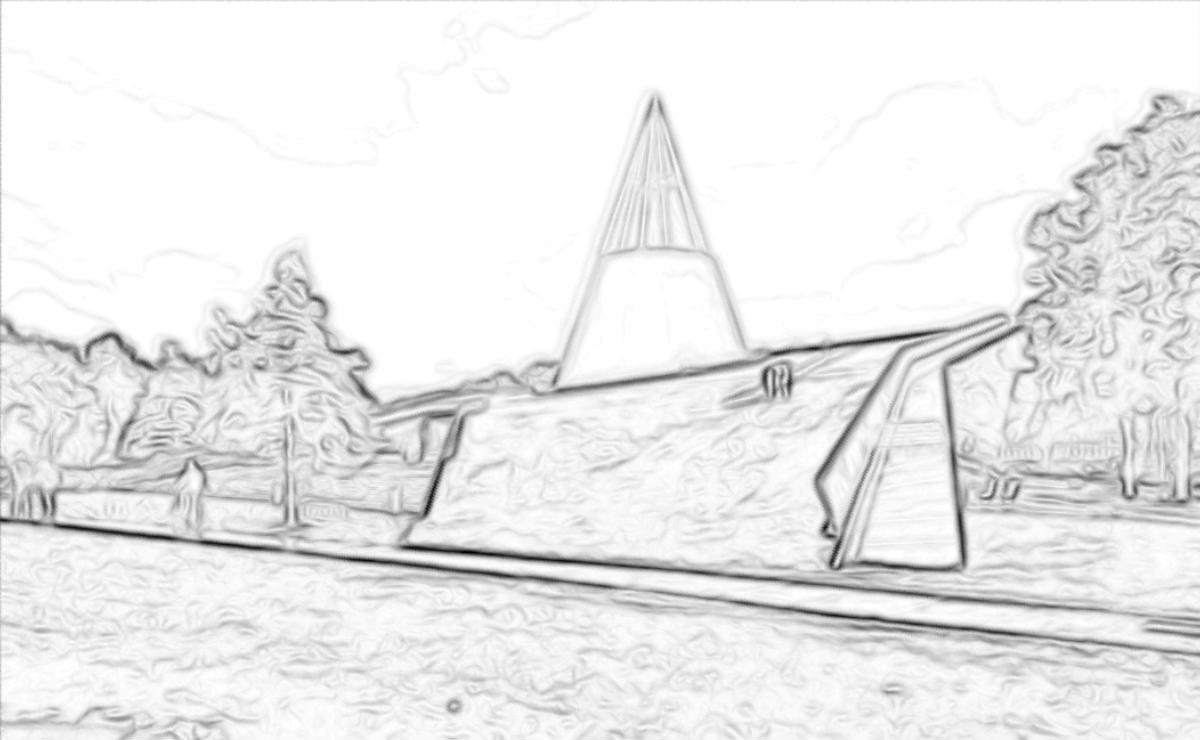
After Watershed Transform
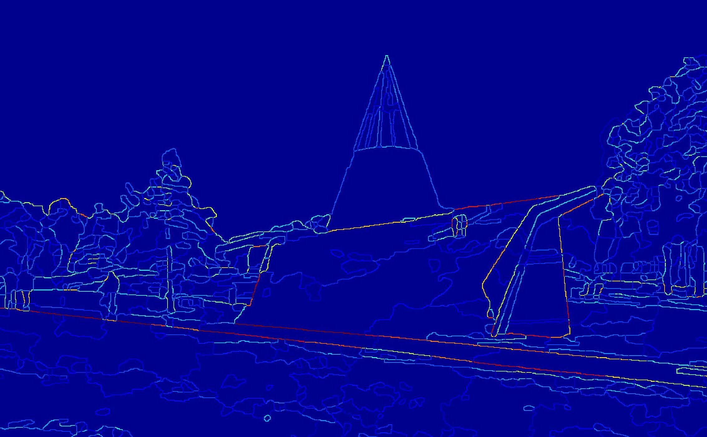
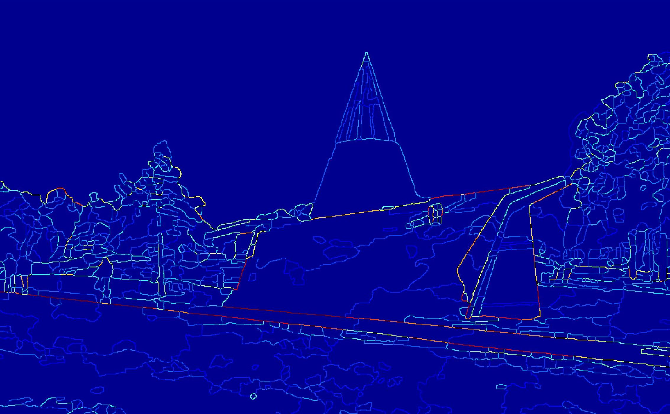
After Oriented watershed Transform (weak boundaries are eliminated)
(click and enlarge the two watershed images to see the difference)
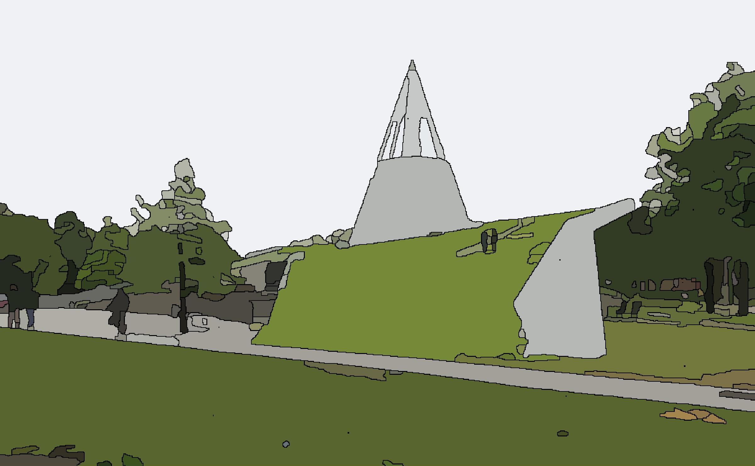
Final image after segmentation